CoursesSystem design from first principles to design review
Puzzle 12 · 13 of 19
Is the database slow, or is the request waiting to reach it?
Connect a user-facing objective to a concrete trace.
All puzzles in this course
The problem
Count requests in flight and watch the waiting queue as you investigate. CPU usage looks healthy. Drivers wait two seconds. The team wants a larger database. What observation could separate a slow query from a wait for a connection?
See it
Scroll sideways to see the full diagram.
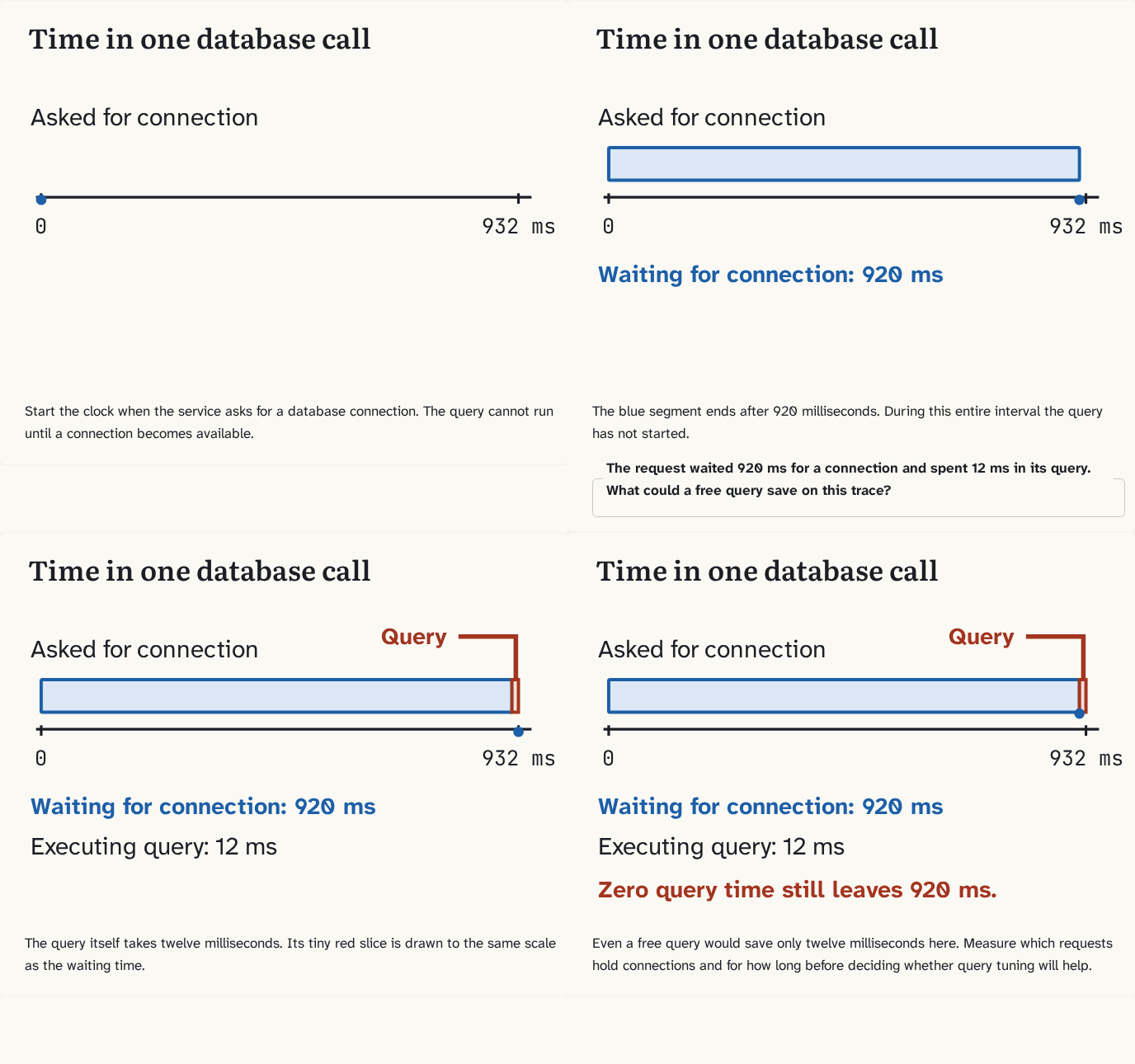
Start the clock when the service asks for a database connection. The query cannot run until a connection becomes available.
Step 1 of 4The blue segment ends after 920 milliseconds. During this entire interval the query has not started.
Step 2 of 4The query itself takes twelve milliseconds. Its tiny red slice is drawn to the same scale as the waiting time.
Step 3 of 4Even a free query would save only twelve milliseconds here. Measure which requests hold connections and for how long before deciding whether query tuning will help.
Step 4 of 4
The building block
Define a service-level objective from the driver's perspective. In a rolling thirty-day window, suppose 99.9 percent of well-formed attempts must return a correct business result within 500 milliseconds. A timely refusal for a full lot meets this contract. A lost reply, server error or two-second success consumes the error budget. With exactly one million attempts, the budget is one thousand bad attempts.
Measure connection wait and query execution separately. In one trace, 920 milliseconds pass before a connection becomes available and twelve inside the query. A missing index is a poor first explanation of that trace. Inspect busy connections and how long requests hold them. If the program waits on another service inside an open transaction, adding connections may simply move the bottleneck.
Measure how quickly the budget is being spent
The objective allows 0.1 percent bad attempts. A five-minute window contains 20,000 attempts and 200 bad outcomes. The observed bad fraction is 1 percent, ten times the permitted fraction. That ratio is the burn rate. If future traffic and failures stay at that proportion throughout a fresh 30-day window, it would use the budget in about three days.
Inspect the same signal across a short and a longer window to separate a persistent incident from a brief spike. Then challenge the diagnosis. If slow traces consistently show connection acquisition under two milliseconds and query execution near one second, investigate the query path. The earlier 920-millisecond wait example called for a different investigation.
Go deeperHow do you compare two releases?
Send a small, representative group to a new version and keep a control group. Measure correct replies within the deadline, write failures and connection saturation. Comparing a new version at rush hour with an old version overnight mixes traffic and software effects. Decide the stopping threshold and check that the old version can still read new data.
One group handles only empty lots. Is its write duration representative of hot lots?
No. Contention and the proportion of refusals change the work.
Find the missing 900 milliseconds
A trace records four timestamps on the same clock. The request begins, a connection becomes available, the query finishes, and the response reaches the measurement boundary. Each request asks for a connection at arrival and starts its query immediately upon acquisition. Both examples finish in 950 milliseconds. Predict which one a faster query could materially improve.
CREATE TABLE trace (
  request TEXT, arrived INTEGER, acquired INTEGER,
  query_done INTEGER, replied INTEGER
);
INSERT INTO trace VALUES
  ('A', 0, 920, 932, 950),
  ('B', 0,   2, 932, 950);

SELECT request,
       acquired - arrived AS wait_ms,
       query_done - acquired AS query_ms,
       replied - query_done AS rest_ms,
       replied - arrived AS total_ms
FROM trace ORDER BY request;Request A spent 920 milliseconds waiting and 12 executing. Holding the other intervals fixed, even an instant query would save at most 12 milliseconds from that trace. Request B spent 930 milliseconds executing. A shared total concealed two different investigations. Change B's acquisition time to 902 while keeping its end time fixed. Which measurement would you now collect first?
These intervals are adjacent and use one clock. A trace containing parallel downstream calls is different. Summing both durations would count their overlap twice. Trace the chain that actually delayed the response.
Try it
Sort one hundred latencies: ninety-eight at 40 milliseconds and two at 2,000. The nearest-rank 99th percentile is observation 99, or two seconds. The mean is 79.2 milliseconds. Design an alert for rapid budget consumption and name one observation that would disprove your first diagnosis.
Check yourself
Sources
- Google SRE · Implementing SLOs — “a target level for the reliability of your service”
What you now know
Separate time spent waiting for a connection from time spent executing a query.
Answer every question above correctly to unlock the next puzzle.
A trace helps diagnose delay. How would you verify the right data survived a restore?
Something wrong or unclear on this page? Tell me: a puzzle that didn't click is a bug in the puzzle.